Hi, Juan!
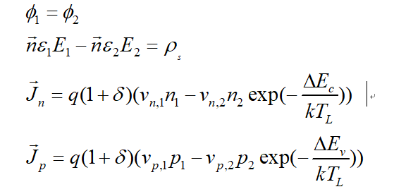
Sorry to bother you. I am trying to simulate a GaN/AlGaN HEMT. And I need to add an interface condition like this, how can I achieve this?
Hi @ghost,
The easiest way I can think of is to add a charge density model to a region on either side of the interface, and to add it to the Potential equation. This may be easiest for the Insulator, if it does not already have a node model assigned to it.
For example create a surface_charge node solution in the insulator and then add this equation:
ElectronCharge * surface_charge * SurfaceArea / NodeVolume
for a surface density \text{cm}^{-2}. SurfaceArea is a node model representing the interface surface area for each node in a region.
Hi, Juan, thanks for your reply.
But I am still confused about the code implementation. Do you mean adding node solutions to the bulk equation or the interface equation?
If in the bulk equation ,according to my understanding, I make such change like this:
def CreatHeterojunctionPotentialOnly(device, region):

    if not InNodeModelList(device, region, "Potential"):
        print("Creating Node Solution Potential")
        CreateSolution(device, region, "Potential")
    elec_i = "n_i*exp(Potential/V_t_T)"
    hole_i = "n_i^2/IntrinsicElectrons"
    charge_i = "kahan3(IntrinsicHoles, -IntrinsicElectrons, NetDoping)"
    Sheet_charge="-ElectronCharge * surface_charge * SurfaceArea / NodeVolume"
    pcharge_i = "ifelse(SurfaceArea > 0,Sheet_charge,-ElectronCharge * IntrinsicCharge)"


    for i in (
        ("IntrinsicElectrons", elec_i),
        ("IntrinsicHoles", hole_i),
        ("IntrinsicCharge", charge_i),
        ("Sheet_charge", Sheet_charge),
        ("PotentialIntrinsicCharge", pcharge_i)
    ):
        n = i[0]
        e = i[1]
        CreateNodeModel(device, region, n, e)
        CreateNodeModelDerivative(device, region, n, e, "Potential")
        CreateNodeModelDerivative(device, region, n, e, "Temperature")

    for i in (
        ("ElectricField",     "(Potential@n0-Potential@n1)*EdgeInverseLength"),
      ("PotentialEdgeFlux", "Permittivity * ElectricField")
    ):
        n = i[0]
        e = i[1]
        CreateEdgeModel(device, region, n, e)
        CreateEdgeModelDerivatives(device, region, n, e, "Potential")

    equation(device=device, region=region, name="PotentialEquation", variable_name="Potential",
             node_model="PotentialIntrinsicCharge", edge_model="PotentialEdgeFlux", variable_update="log_damp")
The object material is not insulator, so I think use “ifelse” can be helpful?However, if add this in the bulk equation, The final assembled equation doesn’t seem to be the equation I want either. It won’t use the parameter in the two sides of interface and make subtraction.
Regarding the interface model, I’m sorry that I don’t know how to assemble the corresponding equations into the interface. I only know how to set up a continuous interface, and I’d be grateful if you could take the time to give an example.
Besides, I also encountered another problem. In addition to setting the potential related to the interface, in order to simulate the heterojunction, the current at the interface also needs to use the thermal electron emission model. He needs to assemble the following interface node model:
This is somewhat similar to the previous question, but I think it needs to be assembled into the continuity equation.
Hi @ghost
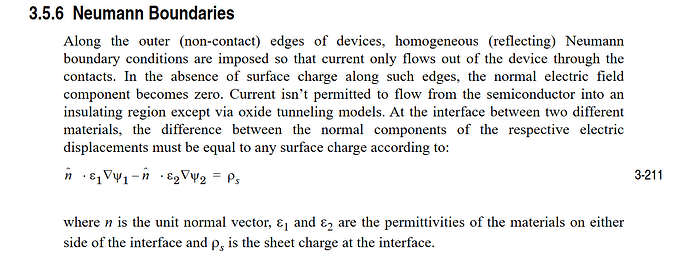
For the “continuous” interface, the bulk equations are added together into the same row of the simulation matrix. This works with your equation 3-211 above, since the surface normals \hat{n} are actually pointing in opposite directions away from the interface.
I am not sure what you mean about having subtraction. Are you saying that opposite signed sheet charges are being placed at each side of the interface?
Would the thermionic emission model take care of the existence of the sheet charge, or is the charge actually specified?
Please see these posts where I try to explain the different modes:
Interface equation for tunneling current
Could the more information can be offered about fluxterm in interface_equation
If it turns out neither of these interface options work for you, there is also the capability to create custom matrix entries that get added to the simulation.
How to use the function custom_equation/
My suggestion is to keep the Potential equation as “continuous”, since the voltage should be continuous across the interface.
For the thermionic emission, have both electrons and holes use the “fluxterm” condition.
If charge still needs to be added, use the custom equation to add it.
These papers have been helpful to my development of the interface modeling:
A Method for Unified Treatment of Interface Conditions Suitable for Device Simulation
https://in4.iue.tuwien.ac.at/pdfs/sispad1997/00621365.pdf
https://doi.org/10.1109/SISPAD.1997.621365
Numerical modeling of heterojunctions including the thermionic emission mechanism at the heterojunction interface
https://doi.org/10.1109/16.52447
Additional Reference:
https://www.iue.tuwien.ac.at/phd/palankovski/node30.html#SECTION001116600000000000000
Hi, Juan. I am really appreciated for your careful and comprehensive reply.
I apologized for my loose expression of the “subtraction”. I mean if adding surface charges in the region equation like I do above to assemble the equation does not reflect the use of dielectric displacement vectors on both sides of the interface. So the “minus sign” in the interface equation may be not reflected:

Moreover, the thermionic emission model may not reflect the sheet charge. In the calculation here, the sheet charge is obtained through polarization and two-dimensional electron gas density, which is a constant.
Through your information and my own learning, I think the final equations that needs to be built in the interface should be:

The first equation represent the continuous of Potential. The second equation reflects the law of Gauß. The last two equation is the thermionic emission model.
I’m sorry, I didn’t study the source code of Devsim in depth, which made me not understand the deep level of equation assembly.I don’t know the specific form of the matrix established by the simple_physicals internal function. My way of understanding is simply to correspond each item in the physical equation to each input item in the equation assembly function. Below I will introduce my thoughts and attempts in detail.If you have time, I beg you to help me correct my mistakes.
The “continuous” is existed in the origin code. I am trying to use the “fluxterm” condition to assemble the sheet charge related and thermionic emission equations.
I am not sure about the meaning of the each term in the “fluxterm”:

The E_n0 seems to represent the equation assembled on node 1? Does F_n correspond to the edge_model in the equation? For example, if the equation I add at the node is assembled into the electron continuity equation, does F_n represent the current density J_n at this time?
According to my understanding, I try to use this to achieve the emission model:
def CreateHeterojunctionInterface(device, interface):
    set_parameter(device=device, name="surface_charge", value=ns)
    set_parameter(device=device, name="Delta_tunneling",   value=0)
    set_parameter(device=device, name="Delta_Ec",   value=0.3766)
    set_parameter(device=device, name="Delta_Ev",   value=0.1614)

    model_name = CreateContinuousInterfaceModel(device, interface, "Potential")
    interface_equation(device=device, interface=interface, name="PotentialEquation", interface_model=model_name, type="continuous")

    Therma_Em_expn="ElectronCharge*(1+Delta_tunneling)/NodeVolume*(An@r0*(Temperature@r0)^2/(ElectronCharge*nstate_density@r0)*Electrons@r0-\
        An@r1*(Temperature@r1)^2/(ElectronCharge*nstate_density@r1)*Electrons@r1*exp(-Delta_Ec/(boltzmannConstant*Temperature@r0/ElectronCharge))"

    Therma_Em_expp="-ElectronCharge*(1+Delta_tunneling)/NodeVolume*(An@r0*(Temperature@r0)^2/(ElectronCharge*pstate_density@r0)*Holes@r0-\
        An@r1*(Temperature@r1)^2/(ElectronCharge*pstate_density@r1)*Holes@r1*exp(-Delta_Ev/(boltzmannConstant*Temperature@r0/ElectronCharge))"

    for name, equation in (
        ("Therma_Em_expn", Therma_Em_expn),
        ("Therma_Em_expp", Therma_Em_expp),
        ("Therma_Em_expn:Electrons@r0", "simplify(diff(%s,Electrons@r0))" % Therma_Em_expn),
        ("Therma_Em_expn:Electrons@r1", "simplify(diff(%s,Electrons@r1))" % Therma_Em_expn),
        ("Therma_Em_expp:Electrons@r0", "simplify(diff(%s,Electrons@r0))" % Therma_Em_expp),
        ("Therma_Em_expp:Electrons@r1", "simplify(diff(%s,Electrons@r1))" % Therma_Em_expp),
        ("Therma_Em_expn:Electrons@r0", "simplify(diff(%s,Temperature@r0))" % Therma_Em_expn),
        ("Therma_Em_expn:Electrons@r1", "simplify(diff(%s,Temperature@r1))" % Therma_Em_expn),
        ("Therma_Em_expp:Electrons@r0", "simplify(diff(%s,Temperature@r0))" % Therma_Em_expp),
        ("Therma_Em_expp:Electrons@r1", "simplify(diff(%s,Temperature@r1))" % Therma_Em_expp),
        ("Therma_Em_expn2", Therma_Em_expn),
        ("Therma_Em_expp2", Therma_Em_expp),
        ("Therma_Em_expn2:Electrons@r0", "simplify(diff(%s,Electrons@r0))" % Therma_Em_expn),
        ("Therma_Em_expn2:Electrons@r1", "simplify(diff(%s,Electrons@r1))" % Therma_Em_expn),
        ("Therma_Em_expp2:Electrons@r0", "simplify(diff(%s,Electrons@r0))" % Therma_Em_expp),
        ("Therma_Em_expp2:Electrons@r1", "simplify(diff(%s,Electrons@r1))" % Therma_Em_expp),
        ("Therma_Em_expn2:Electrons@r0", "simplify(diff(%s,Temperature@r0))" % Therma_Em_expn),
        ("Therma_Em_expn2:Electrons@r1", "simplify(diff(%s,Temperature@r1))" % Therma_Em_expn),
        ("Therma_Em_expp2:Electrons@r0", "simplify(diff(%s,Temperature@r0))" % Therma_Em_expp),
        ("Therma_Em_expp2:Electrons@r1", "simplify(diff(%s,Temperature@r1))" % Therma_Em_expp),
        ):
            devsim.interface_model(device=device, interface=interface, name=name, equation=equation)

    devsim.interface_equation(device=device, interface=interface, name="ElectronContinuityEquation", interface_model="Therma_Em_expn2", type="fluxterm")
    devsim.interface_equation(device=device, interface=interface, name="HoleContinuityEquation", interface_model="Therma_Em_expp2", type="fluxterm")
I use the NodeVolume to represent the integral in the node model, I am not sure if it is reasonable. In this part of the code I give, does I successfully use devsim to create “j=Therma_Em_expn” in the “fluxterm” condition? Since I am confused about F_n, I am not yet sure what form of equation I have assembled.
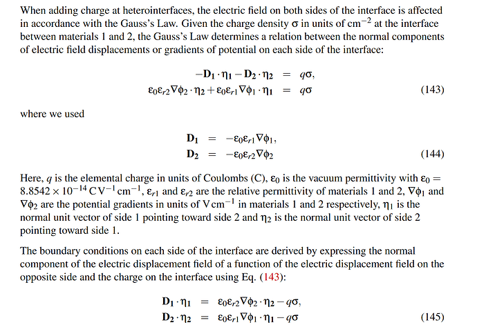
For the sheet charge related equation, I found another TCAD simulator “Charon” write this in its guide book:
The equation (145) own closed form with the “fluxterm” condition. Is it possible to assemble this interface condition using “fluxterm” condition as well? The sheet charge σ(or ρ_s) is a constant. If I want to assemble it into the Poisson’s equation, does F_n in the “fluxterm” condition represent the electric field strength E(▽Φ) ?
Thanks again for replying and helping me.
Hi @ghost
I need a moment to think about what you are working with. I should be adding additional comments throughout the day.
It appears that Charon may have the same node for both materials at the interface, while devsim has a unique node for each material at the interface.
Charon is an FEM solver, which uses some special methods to handle the currents in semiconductor simulation. devsim is an FVM solver, which is actually handling all of the equations in an integral form. This is further described in section II of this paper:
https://www.techrxiv.org/doi/full/10.36227/techrxiv.14129081.v3
Unfortunately the paper does not discuss the interface assembly.
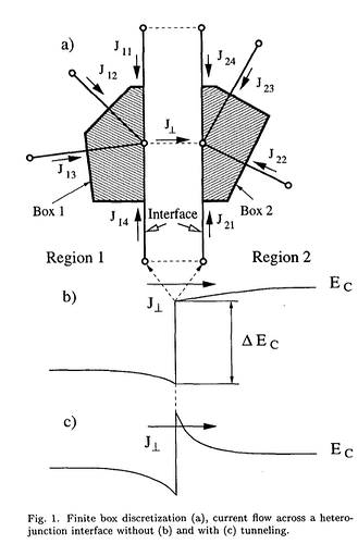
From one of the paper I referenced earlier in this topic (Simlinger et al), this is a nice figure of what the normal component at the interface means:
where J_\perp is equal to the net flux traveling into the next material.
So for the “continuous” interface condition for devsim for the two coincident nodes in different regions: We start with the bulk equations:
where i is the node at material 1 and j is the node at material 2. k and l index adjacent nodes in the same region.
If there is flux between them, this can be stated:
For the continuous boundary condition, these two equations are placed together and an additional 1 is added.
However another equivalent form is keeping the first form with:
where A is a very large number. This would be like an infinite surface recombination velocity.
So back to my notation from this post
Could the more information can be offered about fluxterm in interface_equation
F_{n@r0} and F_{n@r1} comprise of both the node and edge model components being solved in the bulk.
Hi Juan,I really appreciate your detailed response and explanation. I now have a deeper understanding of the interface equations in DEVSIM.
For any interface ( Insulator-Insulator Interface, Semiconductor-Semiconductor Interface … ), it seems necessary to ensure the continuous of both the electric potential and the electric displacement vector at the interface. This is reflected in the reference material you provided:
https://www.iue.tuwien.ac.at/phd/palankovski/node30.html#SECTION001116600000000000000
However, in the presence of interface charges, the electric displacement vector is not continuous but exhibits a jump.
In the format used by DEVSIM to handle continuous boundary conditions at interfaces, as you presented, it appears that the continuity of the interface electric potential is considered (ensured by the second equation), and the continuity of the electric displacement vector at the interface (which should correspond to the first equation, although I’m still a bit confused about the direction of F_Φ. For F_Φ on each interface, are their directions always pointing towards the opposite interface?).
I need some time to organize my thoughts and then consider how to assemble the equations with interface charge using the fluxterm condition.
Thank you again for your help.
F_{\psi_i} is the net flux entering node i from all adjacent nodes in region 1.
F_{\psi_j} is the net flux entering node j from all adjacent nodes in region 2.
For a bulk node during a dc simulation:
If nodes i and j are at the same physical location, I can set up an interface boundary condition.
If I use the “continuous” boundary condition, I use the equations for nodes i and j as:
where the first equation is the net flux entering both nodes, and the second equation is my interface node model.
I hope this helps to resolve the issue you are seeing.
Now if I consider the “hybrid” boundary condition, I can then consider:
to still be true. However the interface model then becomes:
where J_{\perp_{i,j}} is my interface node model and \text{SurfaceArea}_{i,j} is the surface area at the interface.
This can be shown to be equivalent to the “fluxterm” boundary condition:
Hi, Juan.
I organized my thoughts and summarized the implementation method.
For convenience, I upload the note in Github:
I find that your first suggestion can solve the problem of the surface charge exactly. But I didn’t understand how the interface conditions were set before.Sorry for any mix-up that caused. Now I think I know how to set the corresponding interface conditions. If you find any problems or mistakes after reading my note, please tell me. And I will share the code after I verify the correctness of the simulation.
Thank you, Juan, appreciate all your help and patience!
And I want to ask if the interface_model in the “fluxterm” condition is equal to the J_(⊥i,j)?
devsim.interface_equation(device=device, interface=interface, name="ElectronContinuityEquation", interface_model="Therma_Em_expn2", type="fluxterm")
I find there is only one function (devsim.interface_model) to create model in interface. So I want to confirm how to set the J_(⊥i,j) in the “fluxterm” interface condition.
Thanks for sharing your document. I have not done a HEMT simulation before, but I your derivation looks good to me. The interface node model is J_{\perp_{i,j}} an example of this is in:
The ordering of r0, r1 is the same order as devsim.get_interface_list
Hi, Juan!
I have been trying the HEMT simulation for some weeks. I think I’ve completed physics-related modeling refereed to Silvaco Guide book and some articles. However, the program appears to not converge for now. I have check the code for many times but no obvious errors were found. The relative error of the electronic continuity equation in the current program is always stable within a range, about 1e-5. I upload my code in Github:
https://github.com/ZhenglaiT/HEMT-simulation
I really hope you can help me debug the program, especially if you are also interested in HEMT simulation.
Wish you a good day.
Hi @ghost,
I am trying to run your script, gmsh_HEMT2d-Tconst.py on Linux, but it seems like there is some information modifying. After modifying the scripts, (Adding V_t), and fixing the imports, I can get it to finish the equilibrium simulation. Proceeding further in the script, I see there are many missing derivative models:
Could not find or evaluate a model by the name of Temperature:Holes@r1, using 0.0
Could not find or evaluate a model by the name of pstate_density:Holes@r1, using 0.0
Could not find or evaluate a model by the name of Temperature:Electrons@r0, using 0.0
Could not find or evaluate a model by the name of nstate_density:Electrons@r0, using 0.0
on each iteration.
If these models are in fact 0, I highly recomemnd setting them to 0 so that they do not create too many messages in the simulation. In addition, if you change original scripts in python_packages, I recommend changes the script names so it does not create confusion in the output.
Please note that a model like nstate_density:Electrons@r0 means the node model for nstate_density:Electrons in region 0.
I also suggest renaming any of the files you copied from python_packages, so it is easier to see your modifications.
I also see that there must be something wrong with the ElectronContinuity derivatives since the Absolute Error keeps increasing.
I will see if I can look at it a little more before this weekend. I will make a pull request for the files I have edited so far.
You can also print out the symbolic result of a model expression using print()
    x = interface_model(device=device, interface=interface, name=name, equation=equation)

    print(x)


