could the more information can be offered about fluxterm in interface_equation? what about the hybrid?
Hi @fendou1997, thank for your interest in the project. The fluxterm and hybrid are equivalent, but slightly different in the implementation. Unfortunately, the documentation is not clear on this topic, but should be improved in the future.
The added fluxterm is integrated with respect to the interface surface area to one side of the interface and subtracted to the other. It is based on node model values on both sides. This would be good for a model like tunneling across a heterojunction.
Here are the three interface models:
continuous
E_{n0} = F_{n@r0} + F_{n@r1} \\
E_{n1} = C_{r0,r1}
The first equation sums contributions from both the first and second region. The second equation is used to constrain nodal values on both sides. For example, enforcing continuous potential.
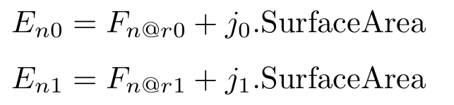
fluxterm
E_{n0} = F_{n@r0} + j \cdot \text{SurfaceArea} \\
E_{n1} = F_{n@r1} - j \cdot \text{SurfaceArea}
where j is the flux across the boundary and is added to the equation in the first region, and subtracted from the equation in the second region. This flux term is based on nodal quantities on both sides of the interface. It is integrated with respect to the surface area at the interface.
hybrid
E_{n0} = F_{n@r0} + F_{n@r1} \\
E_{n1} = F_{n@r1} - j \cdot \text{SurfaceArea}
Models from both regions are summed together. The second equation sets the models in the second region equal to the fluxterm. It is equivalent to the fluxterm formulation.
If this does not fit with what you are trying to do, there is the option to do a Custom Matrix assembly, where you are able to add arbitrary terms to the simulation matrix and right hand side.
Thank you very much. I will try this method and share my example in the future!
1 Like
Thank you for the information on these interface models.
Is it possible to add a different flux to the first region than is subtracted from the second region?
Something like:
This should be possible by using the custom_equation command. The equation is assembled into the simulation matrix on each iteration. In this example, a callback is used to assemble continuous potential across two contacts with coincident nodes in adjacent regions.
It should be possible to do something similar by finding the coincident nodes on both sides of the interface and doing the proper assembly. The SurfaceArea node model is available for doing the surface integration on an interface. The coordinate_index model is used below to find the coincident nodes in each region.
def attach_oxide_contacts():
    fixpot = { }
    ox_coordinates = ds.get_node_model_values(device=device, region="oxide", name="coordinate_index")
    si_coordinates = ds.get_node_model_values(device=device, region="bulk", name="coordinate_index")
    for cox, csi in (('source_ox', 'source'), ('drain_ox', 'drain')):
        csets = []
        csets.append(set())
        csets.append(set())
        for i in ds.get_element_node_list(device=device, region="oxide", contact=cox):
            csets[0].update(i)
        for i in ds.get_element_node_list(device=device, region="bulk", contact=csi):
            csets[1].update(i)
        cmap = {}
        for i in csets[0]:
            cindex = ox_coordinates[i]
            cmap[cindex] = [i]
        for i in csets[1]:
            cindex = si_coordinates[i]
            cmap[cindex].append(i)
        fixpot[(cox, csi)] = cmap


    def myassemble(what, timemode):
        rcv=[]
        rv=[]
        if timemode != "DC":
            return [rcv, rv]

        oxeq = ds.get_equation_numbers(device=device, region="oxide", variable="Potential")
        sieq = ds.get_equation_numbers(device=device, region="bulk", variable="Potential")

        if  what != "MATRIXONLY":
            oxpo = ds.get_node_model_values(device=device, region="oxide", name="Potential")
            sipo = ds.get_node_model_values(device=device, region="bulk", name="Potential")
            for pair in (('source_ox', 'source'), ('drain_ox', 'drain')):
                cmap = fixpot[pair]
                for i, j in cmap.values():
                    rv.extend([oxeq[i], oxpo[i] - sipo[j]])
        if what !="RHS" :
            for pair in (('source_ox', 'source'), ('drain_ox', 'drain')):
                cmap = fixpot[pair]
                for i, j in cmap.values():
                    rcv.extend(
                        [
                            oxeq[i], oxeq[i], 1.0,
                            oxeq[i], sieq[i], -1.0,
                        ]

                    )
        #print(rcv)
        #print(rv)
        return rcv, rv, False

    # CREATE CONTACT EQUATIONS HERE
    # Add output charge later
    ds.contact_equation(device=device, contact="source_ox", name="PotentialEquation")
    ds.contact_equation(device=device, contact="drain_ox", name="PotentialEquation")

    ds.custom_equation(name="fixpotential", procedure=myassemble)
The reason why a contact_equation is used above is to zero out the bulk equations on the oxide side. A contact to the silicon region already exists and is used to apply an external boundary condition. This is to model a thin contact.
Since you wish to maintain the existing bulk equations, you do not need to use the interface_equation or contact_equation commands.
Thank you for your answer.