The calculated precision of Current

[Tao]

Dear DEVSIM developer,
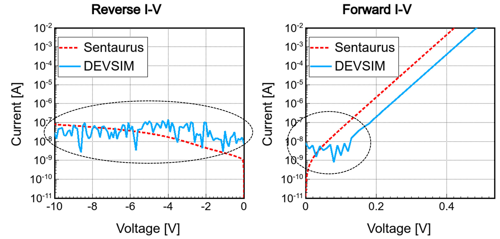
I want to simulate the leakage current of a diode under reverse voltage. But I find there are large fluctuations especially when the leakage current <10^{8} A (see attached figure)， I think it may be dominated by the definition of “error” in solve().

How to simulate the leakage current with higher accuracy?

my script is pasted below:

##############################################################################################################################
# diode_1d.py
##############################################################################################################################

import matplotlib
import matplotlib.pyplot
import math
import csv

device="MyDevice"
region="MyRegion"

CreateMesh(device=device, region=region)

SetParameters(device=device, region=region)
devsim.set_parameter(device=device, region=region, name="taun", value=1e-5)
devsim.set_parameter(device=device, region=region, name="taup", value=1e-5)

SetNetDoping(device=device, region=region)

devsim.print_node_values(device=device, region=region, name="NetDoping")

InitialSolution(device, region)

# Initial DC solution
devsim.solve(type="dc", absolute_error=1.0, relative_error=1e-10, maximum_iterations=30)

DriftDiffusionInitialSolution(device, region)
###
### Drift diffusion simulation at equilibrium
###
devsim.solve(type="dc", absolute_error=1e8, relative_error=1e-10, maximum_iterations=30)



fig1=matplotlib.pyplot.figure(num=1,figsize=(4,4))

x=devsim.get_node_model_values(device=device, region=region, name="x")
fields = ("Electrons", "Holes", "Donors", "Acceptors")
for i in fields:
    y=devsim.get_node_model_values(device=device, region=region, name=i)
    matplotlib.pyplot.semilogy(x, y)
matplotlib.pyplot.xlabel('x (cm)')
matplotlib.pyplot.ylabel('Density (#/cm^3)')
matplotlib.pyplot.legend(fields)
matplotlib.pyplot.savefig("diode_1d_example_density.png")



####
#### Ramp the bias to forward
####
forward_v = 0.0

forward_voltage = []
forward_top_current = []
forward_bot_current = []

forward_voltage.append(0.)
forward_top_current.append(0.)

f1 = open("diode_1d_example_Forward_IV.csv", "w")
header = ["Voltage","Current"]
writer1 = csv.writer(f1)
writer1.writerow(header)

while forward_v < 0.51:

    devsim.set_parameter(device=device, name=GetContactBiasName("top"), value=forward_v)
    devsim.solve(type="dc", absolute_error=1e8, relative_error=1e-10, maximum_iterations=30)
    PrintCurrents(device, "top")
    PrintCurrents(device, "bot")
    forward_top_electron_current= devsim.get_contact_current(device=device, contact="top", equation="ElectronContinuityEquation")
    forward_top_hole_current    = devsim.get_contact_current(device=device, contact="top", equation="HoleContinuityEquation")
    forward_top_total_current   = forward_top_electron_current + forward_top_hole_current       
    forward_voltage.append(forward_v)
    forward_top_current.append(abs(forward_top_total_current))

    writer1.writerow([forward_v,forward_top_total_current])

    forward_v += 0.01

f1.close()


print(forward_voltage)
print(forward_top_current)

fig2=matplotlib.pyplot.figure(num=2,figsize=(4,4))
matplotlib.pyplot.semilogy(forward_voltage, forward_top_current)
matplotlib.pyplot.xlabel('Voltage (V)')
matplotlib.pyplot.ylabel('Current (A)')
matplotlib.pyplot.axis([min(forward_voltage), max(forward_voltage), 1e-9, 1e-2])
matplotlib.pyplot.savefig("diode_1d_example_IV_forward.png")


####
#### Ramp the bias to Reverse
####

reverse_v = 0.0

reverse_voltage = []
reverse_top_current = []
reverse_bot_current = []

reverse_voltage.append(0.)
reverse_top_current.append(0.)

f2 = open("diode_1d_example_Reverse_IV.csv", "w")
header = ["Voltage","Current"]
writer2 = csv.writer(f2)
writer2.writerow(header)

while reverse_v < 10.0:

    devsim.set_parameter(device=device, name=GetContactBiasName("top"), value=0-reverse_v)
    devsim.solve(type="dc", absolute_error=1e4, relative_error=1e-12, maximum_iterations=30)
    PrintCurrents(device, "top")
    PrintCurrents(device, "bot")
    reverse_top_electron_current= devsim.get_contact_current(device=device, contact="top", equation="ElectronContinuityEquation")
    reverse_top_hole_current    = devsim.get_contact_current(device=device, contact="top", equation="HoleContinuityEquation")
    reverse_top_total_current   = reverse_top_electron_current + reverse_top_hole_current       
    reverse_voltage.append(0-reverse_v)
    reverse_top_current.append(abs(reverse_top_total_current))
    writer2.writerow([0-reverse_v,abs(reverse_top_total_current)])
    reverse_v += 0.1

f2.close()

print(reverse_voltage)
print(reverse_top_current)

fig3=matplotlib.pyplot.figure(num=3,figsize=(4,4))
matplotlib.pyplot.semilogy(reverse_voltage, reverse_top_current)
matplotlib.pyplot.xlabel('Voltage (V)')
matplotlib.pyplot.ylabel('Current (A)')
matplotlib.pyplot.axis([min(reverse_voltage), max(reverse_voltage), 1e-9, 1e-2])
matplotlib.pyplot.savefig("diode_1d_example_IV_reverse.png")

[Juan]

Hi @Tao,

For reverse bias, it may be good to try the extended precision mode by placing these lines at the beginning of your script:

devsim.set_parameter(name = "extended_solver", value=True)
devsim.set_parameter(name = "extended_model", value=True)
devsim.set_parameter(name = "extended_equation", value=True)

On the macOS, Linux, and MSYS version on windows, the use of 128 floating point math should improve the solution. A much smaller relative error than 1e-15 may then be achieved.

[Tao]

Hi @Juan ,

Is it possible that I use the “Normalized Units” in DEVSIM to avoid using the “extended_solver”? (such as listed in the table below)


Because I find you use “Real Units Value” in the example code (such as q = 1.6e-19 # coul, k=1.3806503e-23 # J/K, n_i = 1e10 #cm-3), it will easily cause overflow by very large or very small values when solving (or in calculated precision).

[Juan]

Hello @Tao,

Please check to see if extended precision would even help with your device.

I also recommend looking at mesh spacing and other things that could affect accuracy. Perhaps, plot the spatially dependent current and SRH recombination. Also experiment with the Shockley Read Hall model to make sure the lifetimes are appropriate for your device.

It should be possible to use normalized units. You would just need to adjust the model equation scripts appropriately.