Hi all, hi Juan,
I have a question regarding projects based on 2D cylindrical symmetry.
I tried to convert the 2D capacitor example into a project with Cylindrical symmetry using the commands described in the manual.
I thought it would be sufficient to add
ds.set_parameter(name="raxis_zero", value=0) ds.set_parameter(name="raxis_variable", value="x")
ds.cylindrical_node_volume(device=device, region=region)
ds.cylindrical_edge_couple(device=device, region=region)
ds.cylindrical_surface_area(device=device, region=region)
as described in the manual in section 4.6, and then to change the NodeVolumes, EdgeCoupleVolumes and EdgeNodeVolumes with set_parameter() for all the used models.
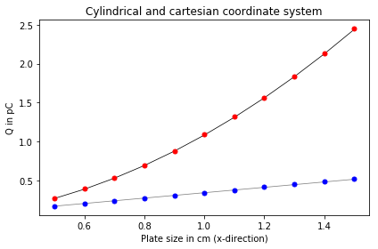
The simulation runs without error, and there are messages indicating a change to a cylindrical coordinate system, but the result (e.g. the contact charge values) are still the same as if I stick to the usual cartesian coordinate system.
I would expect a change in these charge, since the area of the capacitor plates should change in the cylindrical case? Or should they be identical, and I am missing something in the geometry?
Can anyone give me a hint, what I might be doing wrong?
Here is the full code, based on the 2D capacitor example:
import devsim as ds
device="MyDevice"
region="MyRegion"
xmin=-0.5025
x1 =-0.5
x2 =-0.5
x3 =0.5
x4 =0.5
xmax=0.5025
ymin=0.0
y1 =0.1
y2 =0.2
y3 =1.2
y4 =1.3
ymax=5
ds.create_2d_mesh(mesh=device)
ds.add_2d_mesh_line(mesh=device, dir="y", pos=ymin, ps=0.1)
ds.add_2d_mesh_line(mesh=device, dir="y", pos=y1 , ps=0.1)
ds.add_2d_mesh_line(mesh=device, dir="y", pos=y2 , ps=0.1)
ds.add_2d_mesh_line(mesh=device, dir="y", pos=y3 , ps=0.1)
ds.add_2d_mesh_line(mesh=device, dir="y", pos=y4 , ps=0.1)
ds.add_2d_mesh_line(mesh=device, dir="y", pos=ymax, ps=0.5)
device=device
region="air"
ds.add_2d_mesh_line(mesh=device, dir="x", pos=xmin, ps=0.1)
ds.add_2d_mesh_line(mesh=device, dir="x", pos=x1 , ps=0.1)
ds.add_2d_mesh_line(mesh=device, dir="x", pos=x2 , ps=0.05)
ds.add_2d_mesh_line(mesh=device, dir="x", pos=x3 , ps=0.05)
ds.add_2d_mesh_line(mesh=device, dir="x", pos=x4 , ps=0.1)
ds.add_2d_mesh_line(mesh=device, dir="x", pos=xmax, ps=0.1)
ds.add_2d_region(mesh=device, material="gas" , region="air", yl=ymin, yh=ymax, xl=xmin, xh=xmax)
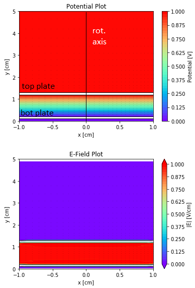
ds.add_2d_region(mesh=device, material="metal", region="m1" , yl=y1 , yh=y2 , xl=x1 , xh=x4)
ds.add_2d_region(mesh=device, material="metal", region="m2" , yl=y3 , yh=y4 , xl=x2 , xh=x3)
# must be air since contacts don't have any equations
ds.add_2d_contact(mesh=device, name="bot", region="air", yl=y1, yh=y2, xl=x1, xh=x4, material="metal")
ds.add_2d_contact(mesh=device, name="top", region="air", yl=y3, yh=y4, xl=x2, xh=x3, material="metal")
ds.finalize_mesh(mesh=device)
ds.create_device(mesh=device, device=device)
###
### Set parameters on the region
###
ds.set_parameter(device=device, region=region, name="Permittivity", value=3.9*8.85e-14)
###
### Create the Potential solution variable
###
ds.node_solution(device=device, region=region, name="Potential")
ds.set_parameter(device=device, region=region,
name="Potential", value="CylindricalNodeVolume")
###
### Creates the Potential@n0 and Potential@n1 edge model
###
ds.edge_from_node_model(device=device, region=region, node_model="Potential")
###
### Electric field on each edge, as well as its derivatives with respect to
### the potential at each node
###
ds.edge_model(device=device, region=region, name="ElectricField",
equation="(Potential@n0 - Potential@n1)*EdgeInverseLength")
ds.set_parameter(device=device, region=region,
name="ElectricField", value="CylindricalEdgeCouple")
ds.edge_model(device=device, region=region, name="ElectricField:Potential@n0",
equation="EdgeInverseLength")
ds.set_parameter(device=device, region=region,
name="ElectricField:Potential@n0", value="CylindricalEdgeNodeVolume@n0")
ds.edge_model(device=device, region=region, name="ElectricField:Potential@n1",
equation="-EdgeInverseLength")
ds.set_parameter(device=device, region=region,
name="ElectricField:Potential@n1", value="CylindricalEdgeNodeVolume@n1")
###
### Model the D Field
###
ds.edge_model(device=device, region=region, name="DField",
equation="Permittivity*ElectricField")
ds.set_parameter(device=device, region=region,
name="DField", value="CylindricalEdgeCouple")
ds.edge_model(device=device, region=region, name="DField:Potential@n0",
equation="diff(Permittivity*ElectricField, Potential@n0)")
ds.set_parameter(device=device, region=region,
name="DField:Potential@n0", value="CylindricalEdgeNodeVolume@n0")
ds.edge_model(device=device, region=region, name="DField:Potential@n1",
equation="-DField:Potential@n0")
ds.set_parameter(device=device, region=region,
name="DField:Potential@n1", value="CylindricalEdgeNodeVolume@n0")
###
### Create the bulk equation
###
ds.equation(device=device, region=region, name="PotentialEquation", variable_name="Potential",
edge_model="DField", variable_update="default")
###
### Contact models and equations
###
for c in ("top", "bot"):
ds.contact_node_model(device=device, contact=c, name="%s_bc" % c,
equation="Potential - %s_bias" % c)
ds.contact_node_model(device=device, contact=c, name="%s_bc:Potential" % c,
equation="1")
ds.contact_equation(device=device, contact=c, name="PotentialEquation",
variable_name="Potential",
node_model="%s_bc" % c, edge_charge_model="DField")
###
### Set the contact
###
ds.set_parameter(device=device, name="top_bias", value=1.0e-0)
ds.set_parameter(device=device, name="bot_bias", value=0.0)
ds.edge_model(device=device, region="m1", name="ElectricField", equation="0")
ds.edge_model(device=device, region="m2", name="ElectricField", equation="0")
ds.node_model(device=device, region="m1", name="Potential", equation="bot_bias;")
ds.node_model(device=device, region="m2", name="Potential", equation="top_bias;")
ds.set_parameter(name="raxis_zero", value=0)
ds.set_parameter(name="raxis_variable", value="x")
ds.cylindrical_node_volume(device=device, region=region)
ds.cylindrical_edge_couple(device=device, region=region)
ds.cylindrical_surface_area(device=device, region=region)
#solve -type dc -absolute_error 1.0 -relative_error 1e-10 -maximum_iterations 100 -solver_type iterative
ds.solve(type="dc", absolute_error=1.0, relative_error=1e-10, maximum_iterations=30, solver_type="direct")
ds.element_from_edge_model(edge_model="ElectricField", device=device, region=region)
#%%
Q_top = ds.get_contact_charge(device=device, contact="top", equation="PotentialEquation")
Q_bot = ds.get_contact_charge(device=device, contact="bot", equation="PotentialEquation")
print('Top contact charge is: '+str(Q_top))
print('Bottom contact charge is: '+str(Q_bot))
#%%
ds.write_devices(file="cap2d.msh", type="devsim")
ds.write_devices(file="cap2d.dat", type="tecplot")
ds.write_devices(file="cap2d", type="vtk")
As always, thank you very much for any help.